R 的資料結構
Wush Wu
國立台灣大學
分析的資料型態:數值系統
數值系統的分類
- 名目資料(nomial)
- 順序資料(ordinal)
- 區間資料(interval)
- 比例資料(ratio)
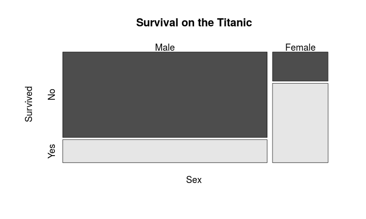
名目資料
- 性別
- Domain
- 屬性的有無
順序資料
- 硬度表
- 名次
- 排序表
[1] Qn1 Qn1 Qn1 Qn1 Qn1 Qn1
12 Levels: Qn1 < Qn2 < Qn3 < Qc1 < Qc3 < Qc2 < Mn3 < Mn2 < Mn1 < ... < Mc1
區間資料
- 溫度
- 時間

比值資料
- 營收
- 股價

R 的資料型態
R 的資料結構概論
- R 是一種程式語言,程式語言都有對應的資料結構
- Rinternals.h:
typedef unsigned int SEXPTYPE;

#define NILSXP       0    /* nil = NULL */
#define SYMSXP       1    /* symbols */
#define LISTSXP      2    /* lists of dotted pairs */
#define CLOSXP       3    /* closures */
#define ENVSXP       4    /* environments */
...
R 的資料結構
- 所有的東西都是一種「R 物件」
- 資料
- 函數
- 環境
- 外部指標
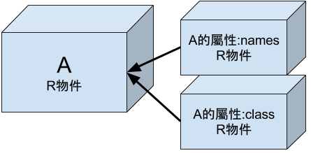
R 的物件結構
- 複雜的R 物件們都是由基礎的R 物件所組合的
g <- lm(dist ~ speed, cars)
str(head(g))
List of 6
 $ coefficients : Named num [1:2] -17.58 3.93
  ..- attr(*, "names")= chr [1:2] "(Intercept)" "speed"
 $ residuals    : Named num [1:50] 3.85 11.85 -5.95 12.05 2.12 ...
  ..- attr(*, "names")= chr [1:50] "1" "2" "3" "4" ...
 $ effects      : Named num [1:50] -303.914 145.552 -8.115 9.885 0.194 ...
  ..- attr(*, "names")= chr [1:50] "(Intercept)" "speed" "" "" ...
 $ rank         : int 2
 $ fitted.values: Named num [1:50] -1.85 -1.85 9.95 9.95 13.88 ...
  ..- attr(*, "names")= chr [1:50] "1" "2" "3" "4" ...
 $ assign       : int [1:2] 0 1
R 的物件結構
R 中常見的原子物件
- 邏輯向量
- 整數向量
- 數值向量
- 字串向量
R 的所有設計都是為了分析資料而生
- 資料的最小單位是「向量」
邏輯向量
- 用於作布林運算、流程控制
c(T, F, TRUE, FALSE)
[1] TRUE FALSE TRUE FALSE
整數向量
- 每個整數佔用4 bytes
c(1L, 2L, 3L, 4L, 0xaL)
[1] 1 2 3 4 10
數值向量
- 每個數值佔用8 bytes(雙精確浮點數)
c(1.0, .1, 1e-2, 1e2, 1.2e2)
[1] 1.00 0.10 0.01 100.00 120.00
字串向量
- NULL結尾的字串向量
c("1", "a", "中文")
[1] "1" "a" "中文"
c("a\0b")
Error: nul character not allowed (line 1)
數值系統與原子資料結構
- 名目資料(nomial): 字串向量、邏輯向量
- 順序資料(ordinal): 無
- 區間資料(interval): 整數向量、數值向量
- 比例資料(ratio): 整數向量、數值向量
習題時間
請同學完成以下的swirl課程,練習操作上述介紹的R 物件
RBasic-02-Data-Structure-Vectors
RBasic-03-Data-Structure-Object
R 的factor
R 的物件結構
內建的factor範例
head(CO2$Type)
[1] Quebec Quebec Quebec Quebec Quebec Quebec
Levels: Quebec Mississippi
factor的真相
dput(CO2$Type)
structure(c(1L, 1L, 1L, 1L, 1L, 1L, 1L, 1L, 1L, 1L, 1L, 1L, 1L,
1L, 1L, 1L, 1L, 1L, 1L, 1L, 1L, 1L, 1L, 1L, 1L, 1L, 1L, 1L, 1L,
1L, 1L, 1L, 1L, 1L, 1L, 1L, 1L, 1L, 1L, 1L, 1L, 1L, 2L, 2L, 2L,
2L, 2L, 2L, 2L, 2L, 2L, 2L, 2L, 2L, 2L, 2L, 2L, 2L, 2L, 2L, 2L,
2L, 2L, 2L, 2L, 2L, 2L, 2L, 2L, 2L, 2L, 2L, 2L, 2L, 2L, 2L, 2L,
2L, 2L, 2L, 2L, 2L, 2L, 2L), .Label = c("Quebec", "Mississippi"
), class = "factor")
factor的真相
attributes(CO2$Type)
$levels
[1] "Quebec"      "Mississippi"

$class
[1] "factor"
R 的歷史包袱
dput函數會輸出如.Label這種標籤,但是並不是真正的屬性標籤以下內容擷取自
structure的說明文件:Adding a class "factor" will ensure that numeric codes are given integer storage mode.
For historical reasons (these names are used when deparsing), attributes ".Dim", ".Dimnames", ".Names", ".Tsp" and ".Label" are renamed to "dim", "dimnames", "names", "tsp" and "levels".
數值系統與資料結構
- 名目資料(nomial): 字串向量、邏輯向量、factor
- 順序資料(ordinal): factor
- 區間資料(interval): 整數向量、數值向量
- 比例資料(ratio): 整數向量、數值向量
習題時間
- 請同學完成
RBasic-04-Factors,練習操作R 的factor物件
R 的Matrix與array
R 的Matrix
> x <- matrix(1:4, 2, 2)
> x
     [,1] [,2]
[1,]    1    3
[2,]    2    4
> class(x)
[1] "matrix"
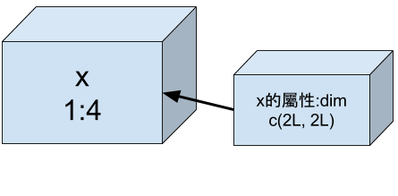
R 的Matrix與Attributes
> attributes(x)
$dim
[1] 2 2
R 的Matrix與Attributes
> attributes(x) <- NULL
> x # 同 1:4
[1] 1 2 3 4
R 的Matrix與Attributes
R 的Array與Attributes
> attr(x, "dim") <- c(2, 2, 1)
> x # 同 1:4
, , 1

     [,1] [,2]
[1,]    1    3
[2,]    2    4
> class(x)
[1] "array"
為什麼要使用R 的Matrix?
- 各種方便操作的API
- 優化過的運算效能(BLAS)
習題時間
- 請同學完成
RBasic-05-Arrays-Matrices,練習操作R 的matrix和array物件
List: R 物件的向量
原子物件向量,具備有同質性
- 牽一髮而動全身
> x <- 1:10
> class(x)
[1] "integer"
> x[1] <- "1"
> class(x)
[1] "character"
> x
 [1] "1"  "2"  "3"  "4"  "5"  "6"  "7"  "8"  "9"  "10"
實務的資料不只是單一型態
- R 物件可以是任何型態的向量
- R 物件的向量就是處理相異型態的工具
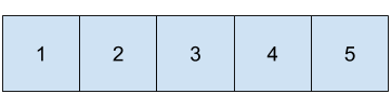
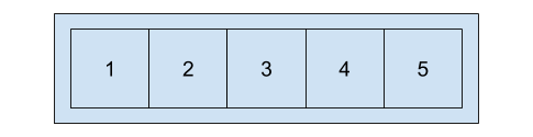
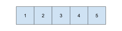
整數向量
1:5
List
x <- list(1:5, c("a", "b"))
[
x[1]
[[
x[[1]]
List and names
> x <- list(1:5, c("a", "b"))
> x
[[1]]
[1] 1 2 3 4 5

[[2]]
[1] "a" "b"

> attributes(x)
NULL
List and names
> x <- list(a = 1:5, b = c("a", "b"))
> x
$a
[1] 1 2 3 4 5

$b
[1] "a" "b"

> attributes(x)
$names
[1] "a" "b"
$
- 取出對應名稱的元素
> x <- list(a = 1:5, b = c("a", "b"))
> x$a
[1] 1 2 3 4 5
> x$b
[1] "a" "b"
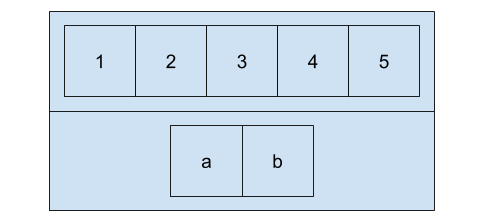
從List到data.frame
- List提供了處理異質資料的工具
- List非常的泛用,甚至延生出R 的S3物件導向系統
- 但是對於結構化的資料,List不夠方便阿...
- 看看矩陣
data.frame是R 為了解決結構化資料所提出的解決方案
R 的 Data Frame
R 的Data Frame
已經成為處理「結構化資料」的典範
The main driver for Distributed DataFrame is to have a cluster-based, big data representation that’s friendly to the RDBMSs and data science community. Specifically we leverage SQL’s table and R’s data.frame concepts, taking advantage of 30 years of SQL development and R’s accumulated data science wisdom.
R 的Data Frame
> head(iris)
  Sepal.Length Sepal.Width Petal.Length Petal.Width Species
1          5.1         3.5          1.4         0.2  setosa
2          4.9         3.0          1.4         0.2  setosa
3          4.7         3.2          1.3         0.2  setosa
4          4.6         3.1          1.5         0.2  setosa
5          5.0         3.6          1.4         0.2  setosa
6          5.4         3.9          1.7         0.4  setosa
Data Frame是一種List
> class(iris)
[1] "data.frame"
> is.list(iris)
[1] TRUE
> head(iris[[1]])
[1] 5.1 4.9 4.7 4.6 5.0 5.4
Data Frame 提供了類似矩陣的API
> iris[1,]
  Sepal.Length Sepal.Width Petal.Length Petal.Width Species
1          5.1         3.5          1.4         0.2  setosa
> iris[1,1]
[1] 5.1
習題時間
- 請同學完成
RBasic-06-List-DataFrame的課程,實際操作List和Data.Frame
實務經驗
記憶體問題
- R 是一個以記憶體為主的分析工具
- R 假設你的記憶體是足夠的
- R 跑得很慢
- CPU 不夠快(計算量太大)
- 記憶體不夠大(資料太大)
如何估計記憶體的使用量?
- 向量就是陣列,加上一些其它的metadata(型態、attributes、...)
- 邏輯向量、整數向量和數值向量的空間大約為:\(長度 \times 單位空間\)
object.size
object.size(logical(0))
40 bytes
object.size(rep(TRUE, 1000))
4040 bytes
object.size(rep(TRUE, 1e6))
4000040 bytes
object.size
object.size(integer(0))
40 bytes
object.size(seq(1L, by = 1L, length = 1e3))
4040 bytes
object.size(seq(1L, by = 1L, length = 1e6))
4000040 bytes
object.size
object.size(numeric(0))
40 bytes
object.size(seq(0, by = 1, length = 1000))
8040 bytes
object.size(seq(0, by = 1, length = 1e6))
8000040 bytes
字串向量的記憶體用量不容易估計
speaker <- readLines("speaker.txt")
speaker[2]
[1] "年會總召, 中央研究院資訊科學研究所/ 研究員"
length(speaker)
[1] 216
file.size("speaker.txt")
[1] 18464
object.size(speaker)
24664 bytes
關於記憶體
- 事前估計需要的記憶體用量
- 抓"0"的個數即可
R 的記憶體處理機制
- 垃圾回收(
gc()) - Pass By Value
- Copy on Write
gc會進行以下動作:
- 釋放不使用的記憶體
- 關閉不使用的檔案連線
Pass By Value
- 在R 的函數中對物件作修改,外部物件是不會被更改的
- 物件被複製了!
Copy on Write
- 只有在修改物件的時候,才會複製記憶體
tracemem
> x <- c(1, 2, 3)
> tracemem(x)
[1] "<0x8de5838>"
> y <- x
> y[2] <- 3
tracemem[0x8de5838 -> 0x7f99070]